Valuation Of Inherent Return Vs. Fiat Return Assets – A Common Principle

© Julian Van Erlach 5/27/22

Economic assets can be classified into two broad categories: those earning an inherent return and those earning a fiat money return. This article shows that both are valued according to the same general principle based on GDP (a constant equal to expected long term real per capita GDP growth) but through mechanisms that depend on the attributes of how they obtain their return. What is NOT factored is any measure of RISK or “risk premium”, or supply and demand “imbalances” – and yet, the models perform extremely well empirically and theoretically using only public, real-time data. Adding risk and supply/demand factors does not improve model performance.

Inherent vs Fiat Return Assets

By inherent return, I mean assets whose supply growth is less than real GDP growth. Stocks and bonds earn their return in the form of fiat money profits and payments. Fiat money supply generally exceeds real GDP growth and is at the whim of governments. Therefore, it loses purchasing power: inflation.

GDP growth can be defined as the sum of population growth, real per capita productivity growth and inflation. Long-term productivity growth was about 2% until the 2008 Financial Crisis after which the rate dropped to about 1% and is projected to remain at that level for quite some time: see Conference Board. (The reason for that has to do with excess capital formation by the government and Fed; by buying bad loans for example. There is research showing that excess money creation is linked to productivity declines; but is beyond the scope of this post.)

Chart 1: (BLS) Per Capita Productivity Growth Rates

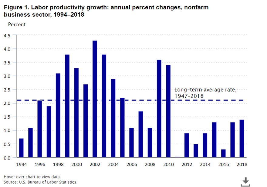
The supply of Bitcoin is capped, the above ground gold stock growth rate (new mine output) grows at the rate of population growth (Charts 2, 3); and the supply and consumption of oil moves directly with population growth (Chart 4).

Charts 2 & 3 (MathewTurner.co.uk) Respectively Rate of Change of World Gold Stock and Absolute Level

Chart 2: Rate of Increase of Gold Stock

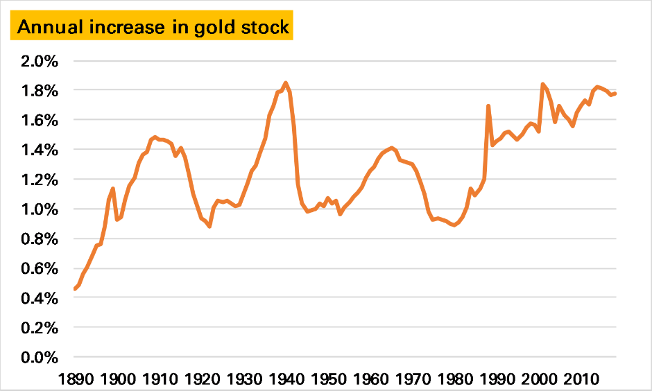
Chart 3: Above Ground Gold Stock

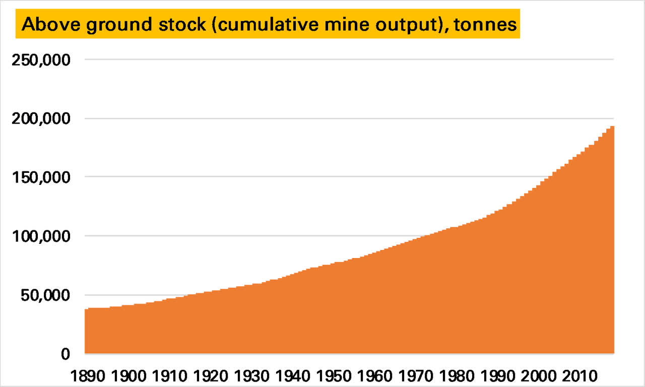
Chart 4: (Earlywarn.blogspot.com) World Oil Consumption per Capita History

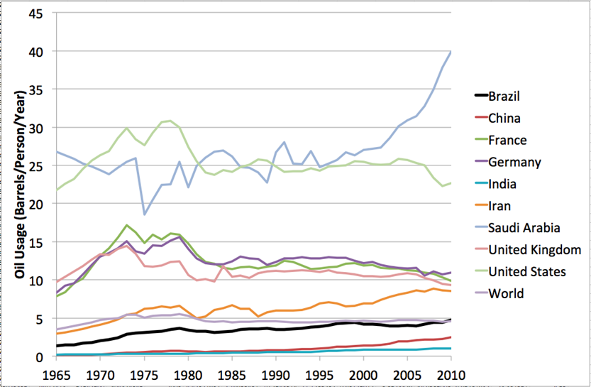
The attributes of fiat money are government control with longer term unpredictable policy actions and supply growth exceeding real GDP growth, which causes loss of purchasing power i.e., inflation: Chart 5.

Chart 5: (author) M3/Real GDP Indexed vs CPI

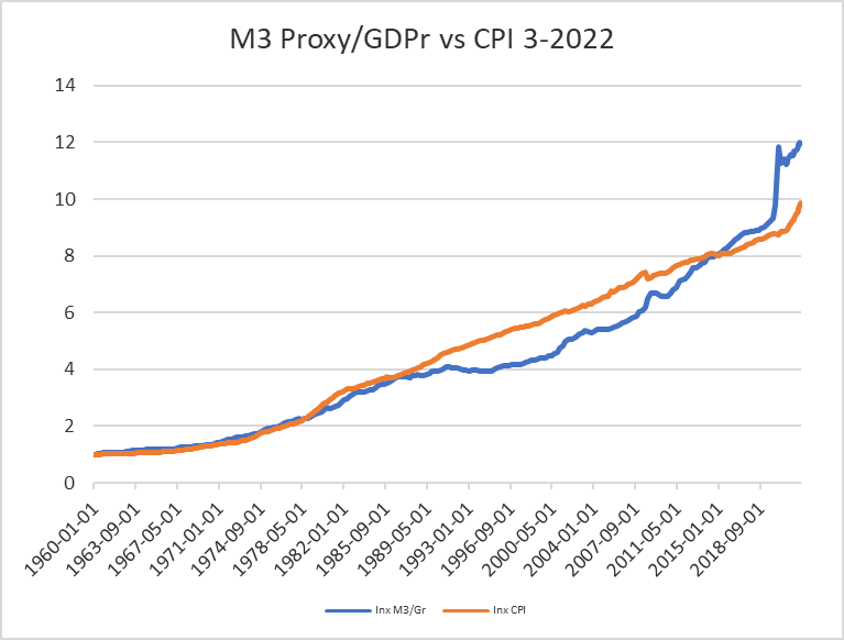
The money supply spike recently caused by the Treasury and Fed (buying bonds/loans with newly created money, creating bank reserves, creating money in the Treasury account so the Treasury can give money to people) can be clearly seen driving the subsequent surge in inflation/loss of money purchasing power in a relationship shown across more than 62 years using St. Louis Fed data. Thus, what gives money value in terms of goods and services is its relationship to real GDP. The same is true for assets which obtain an inherent return. In the case of those assets, world real GDP increases per unit of assets with an inherent (real) return.

The CPI must and will catch up to the excess money supply vs real GDP. Banks aren’t the cause of the excess money supply because if they were, they would report massive loan losses as money loaned out would not be repaid to account for the excess money supply. Without government miss incentives, banks must create loans only with the expectation and realization of spurring real growth and return; else they go under.

Whereas fiat money loses real purchasing power, assets whose stock growth rate is less than real GDP growth gain in real purchasing power as real global GDP per unit increases (gold and Bitcoin) or hold that purchasing power steady over time if the asset enables a constant productivity rate such as oil. In the next section the article will look at why the fiat money prices of assets change.

In addition to causing inflation, excess money supply reduces the possible return on bond investment due to an excess of created supply vs available real return from real GDP output. This can be seen in how excess money supply affects the real yield as measured by TIPS (Treasury Inflation-Protected Securities) Chart 6.

Chart 6A: (author using St. Louis Fed data) Fed Balance Sheet (Money Creation) vs TIPS Yield

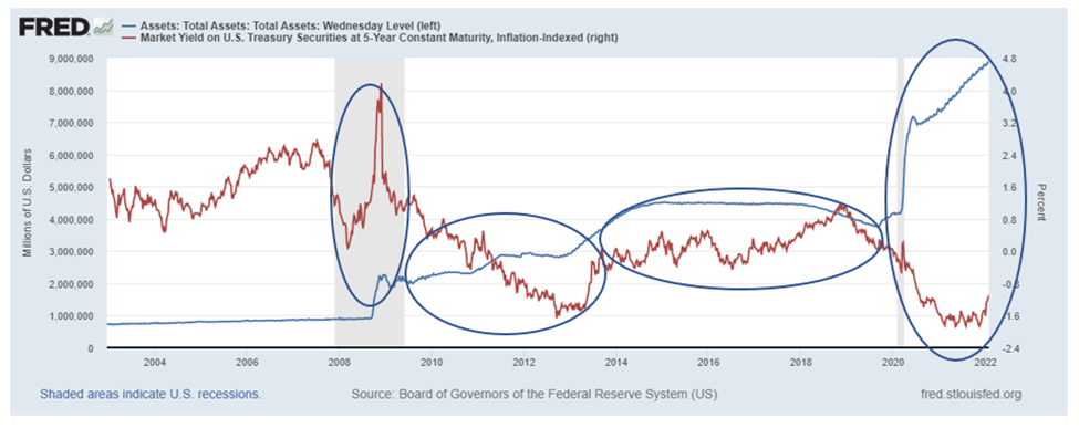
Clearly, excess money creation destroys the ability to earn a real yield, or an adequate real yield on bond investment.

Chart 6B: (Economicshelp.org) UK Example Showing How Excess Money Supply Affects Bond Yield

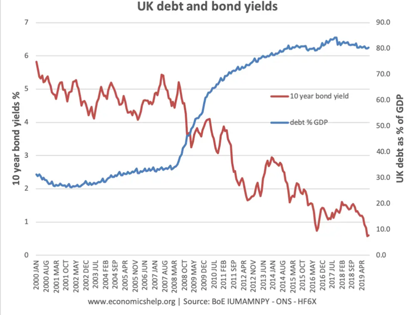
A basic Table 1 shows the relationship of GDP to fiat and inherent return assets:

The table shows that GDP growth is comprised of inflation, productivity, and population growth. The EPS or earnings per share growth of the stock market equals the sum of inflation and productivity growth while share growth equals population growth (these are proven; and not mere assertions, see this paper for a more full discussion and proof that there is no “equity premium” at the market level). The equity premium thesis assumes full dividend yield reinvestment which is infeasible since share growth equals population growth and is much less than the dividend yield – thus there is no equity premium at the market level.

The after-tax long bond yield requires a real return equal to productivity growth unless the money supply is manipulated making this impossible as at present.

Using the above chart, the attributes of many asset classes can be compared to those of GDP growth. Valuation is also a function of GDP growth. Thus, the real economy and the valuation of all assets, fiat, and inherent return, are inextricably linked by mathematically described laws which meet the test of science: an encompassing theory that makes empirically testable predictions.

Fiat Asset Valuation

Long Bond Yield

According to the Required Yield Theory co-developed with Christophe Faugere, the long bond yield should be the pre-tax yield needed to cover expected inflation and tax, resulting in a real after-tax yield equal to long term per capita productivity growth within the term structure of the bond. The essence of the formula which predicts the long bond yield adds the expected inflation rate to the expected long term per capita real GDP growth rate and divides the result by 1 minus the effective tax rate on interest income in a long-term tax-deferred portfolio. To the result, it adds the 5-year TIPS yield if it is below zero. The formula states that bond investors want a real, after-tax interest rate that approximates real per capita GDP growth expected over the term of the bond. This required yield is reduced by the extent of negative TIPS yields which as shown below is caused by an excess of money supply created by the Fed.

In a mature economy not manipulated by the central bank or Treasury, the ratio of total debt to GDP should remain constant; enabling bond investors to earn a real after-tax return equal to real per capita GDP growth within the term of the bond.

Chart 7 shows the predictive and descriptive ability of the formula to model the actual yield.

Chart 7: (author) Predicted vs Actual Average 20-30-year Long Bond Yield

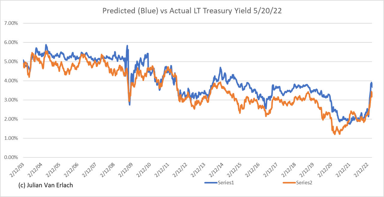
Both inflation and negative real yields are caused by Federal Government policy, and both affect the returns bond investors obtain. Even Treasury investors face real return risks caused by increasing inflation and increased tax rates for example. The return on capital directly limits the real return on labor as well but is beyond the current scope.

Stock Market Valuation

The exact sample principle applies to the stock market: price is determined according to a required real after-tax yield that is equal to long term expected real per capita productivity growth (which is essentially a constant). No so-called equity risk premium is involved. Academics and investment professionals generally hold that stock market valuation involves such a premium. It does not and cannot exist for the reasons discussed above and in the linked paper.

The principle of a required real after-tax (constant) yield equal to long term real expected per capita productivity growth can be applied to stock market valuation: the P/E or price/earnings ratio. In simple form, the P/E must equal 1 /[(expected inflation + expected real long-term per capita productivity growth)/(1 – the expected effective tax rate on tax-deferred investment accounts)] (Formula 1). No risk premium factor. The after-tax dividend yield offsets capital gains taxes (where in the long run, capital gains must equal EPS growth), which leaves real long-term per capita productivity growth as the real after-tax return from the stock market as a whole. There is a price floor, even in the face of very low or negative expected earnings determined by the expected dividend yield, which when equal to the required yield as defined above provides a price floor in such a circumstance.

The assertions above can be further validated by using Fed Funds Flows data showing the increase in stock market value over time and the total dividends paid. If a single entity owned the entire stock market at the starting point and invested dividends, it could only do so in net new shares offered. Thus, in the best case, the compound return attainable would be the growth in stock market value and a large fraction of dividends paid being retained – that return is FAR less than what academics have calculated with the assumption of full tax-free dividend yield reinvestment which is the crux of the equity premium model. In addition, an equity premium implies compound stock market returns that far exceed GDP growth – an impossibility.

Individual investors and tax-free entities can get higher returns by fully reinvesting the dividend yield, but the MARKET as a whole cannot. The market is valued by the market-level return; not what a particular class of investors may be able to obtain.

Chart 8: (author) Shows the Above Formula (Blue) Compared to the Actual 1-Year Forward (Grey) and Trailing S&P 500 P/E

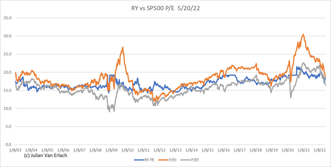
The Blue line is the predicted P/E and the Grey line is the P/E based on 1-year forward expected EPS for the S&P 500.

According to this model, the recent fall in the stock market is mainly caused by rising inflation expectations as measured by the St. Louis Fed 5-Year inflation expectations updated daily. However, the actual forward P/E is more than 10% lower than predicted, likely because of concerns that a recession may occur and pull forward earnings down. A much more detailed discussion is in this published journal paper out of NYU.

Some have claimed that Fed balance sheet expansion has driven stocks higher. Chart 9 shows this is not true, with examples of large increases in the stock market during flat to lower Fed balance sheet levels.

Chart 9: (author) The S&P 500 Has Risen Even When Fed Assets Were Constant or Falling

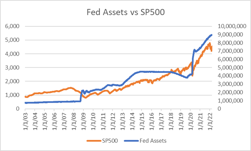
Inherent Return Asset Valuation

This section shows how the same principle values gold, Bitcoin, and oil. I use only US data in this post because I cannot find reliable comparable global data. Oil, gold, and Bitcoin are global assets, and as such driven by the GDP or trade-weighted composite national measures of the data I use as well as supply and demand to a degree. US bonds and stocks are further subject to a degree of arbitrage trading on a global scale. Thus, it is remarkable how accurate at predicting and tracking the values of these assets in US$ the methods in this analysis are. I use the term “prediction” to mean that the model used here accurately predicts the direction and magnitude of price changes of these assets for any given set of future values of the variables used here: expected inflation, expected long term real per capita GDP growth, effective corporate and personal tax rates, expected earnings, the trade-weight exchange rate – all publicly available data. This constitutes a scientific test.

Inherent return assets earn an increasing real return in the case of gold and Bitcoin because real world GDP rises per unit of the outstanding stock of each. Oil which is a flow, earns a constant real return because it enables a constant level of productivity.

Gold

A full discussion of how gold is valued is in this Journal of Investing paper. Because gold obtains an inherent real return per unit, unlike fiat money, its value should be a cumulative function of both global fiat inflation and real per capita GDP growth (since the world gold stock increases at the rate of population growth; therefore world real GDP increases per unit of gold at the rate of real per capita growth – and fiat money loses purchasing power vs gold at its rate of inflation). In addition, its valuation changes will be an inverse function of a local currency value vs a global exchange rate index, an inverse function of the fiat asset real yield as measured by an indicator such as the TIPS or Treasury Inflation-Protected Security yield (as the real yield obtainable by fiat bond investment falls or goes negative, the relative value of gold should rise; for example), and a further direct function of the Required Yield as defined by the denominator in Formula (1) shown in the Stock Market Valuation section (this factor falls as expected inflation falls; pulling down gold because the expected purchasing power of fiat money is falling at a lower rate). Putting all of this together in Chart 10, the “AuRY” line is the applied formula since 2002 vs actual USD$ gold price line “Au”.

Chart 10: (author) Predicted vs. Actual USD$ Gold Price

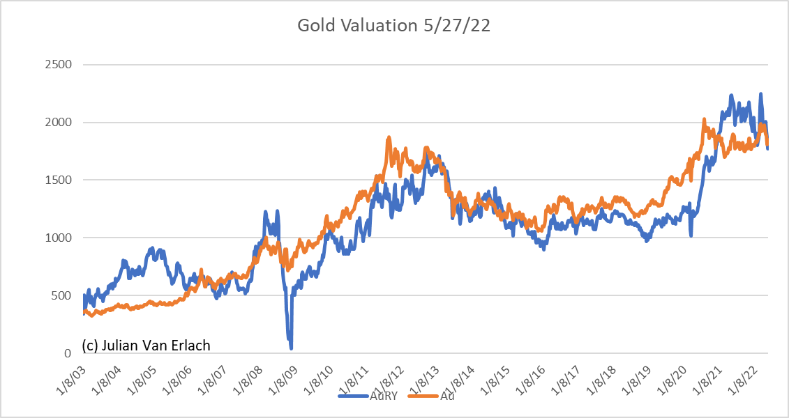
The same model in the cited paper holds just as well during the World true Gold Standard, spanning over 200 years; and fully solves the heretofore unsolved Gibson’s Paradox.

Bitcoin

Bitcoin has been the subject of wild investment swings and massive global government policy changes. Some corporations and investment funds have bought heavily. As in the case for gold, world real GDP is increasing per Bitcoin because of constrained and soon-to-be capped supply. Therefore, all of the above valuation variables apply for Bitcoin as well. In the example below, I use the resulting yield created from the formula: [(expected inflation + expected real long-term per capita productivity growth)/(1 – the expected effective tax rate on tax-deferred investment accounts)] – TIP 5-Year (real) yield. The first part of the formula is just the denominator of Formula (1). The real yield is subtracted, which if negative, adds to the yield in the formula. Thus, Bitcoin is expected to move up with an increasingly negative real yield as stated previously. This formula models the price movement of Bitcoin very well and is theoretically consistent with the valuation approach described here.

Chart 11: (author) Predicted vs Actual Bitcoin Price Movements

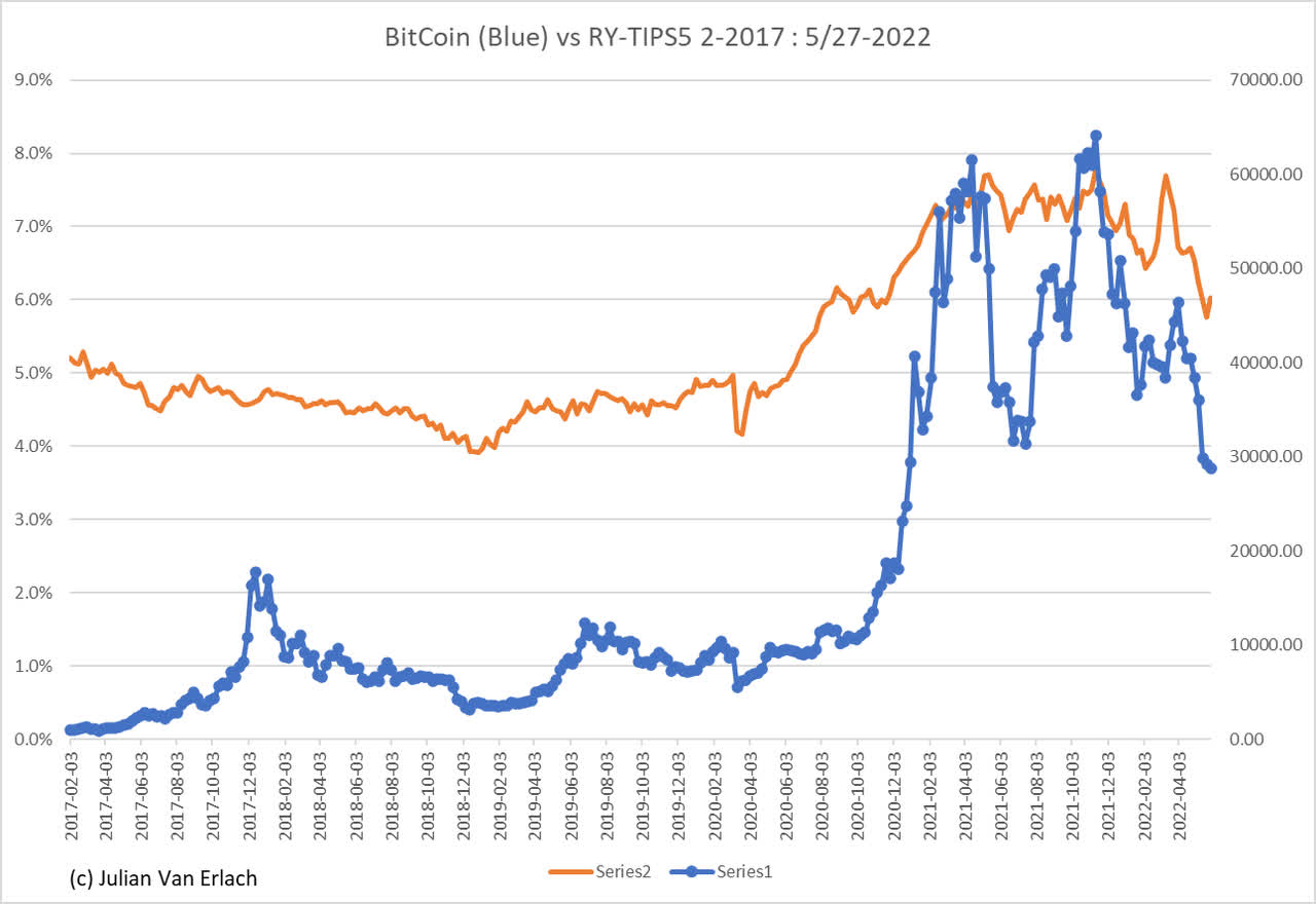
Chart 12: (Coindesk.com): Investment Inflows Coincide with Valuation Jump

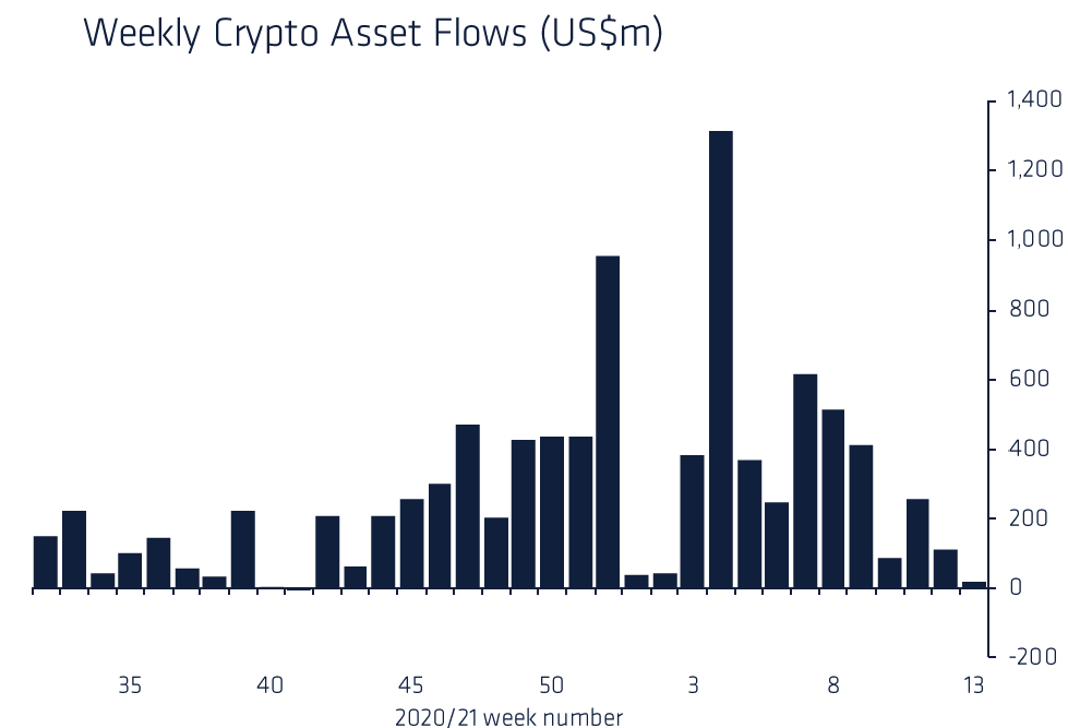
It is clear that the price spike of late 2020-21 was driven by investment inflows and has increased price volatility. Despite those flows, and the global nature of the asset, my proposed model describes the actual valuation changes extremely well using just US data. The implication is that much of current valuation is not fundamentally substantiated and the decline of expected inflation coupled with rising real yield if realized, are and will continue to be catastrophic for Bitcoin in the near term, but not long term.

Oil

Chart 13A: (author) Predicted vs Actual USD$ WTC Oil Price

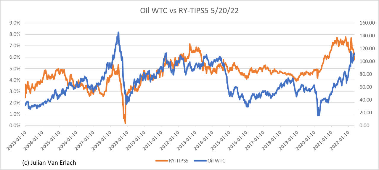
Oil is of course also a global commodity, and a flow rather than a stock, which gold and bitcoin are. As a global commodity, it is influenced by supply/demand fluctuations, political events, and other global financial factors. The simple version of the formula used in Chart 13A is exactly the same as for Bitcoin and part of gold valuation. Clearly, these assets share economic characteristics. The difference is that oil does not gain real value with real world per capita GDP growth, whereas gold and Bitcoin do.

Note that in Chart 13B, showing the price of oil vs supply and demand imbalances, that during 2004-05, the price of oil rose in the face of excess supply, and then fell in the face of a deficit in early 2006. This directly corresponds to what the model predicts, despite the contrary supply/demand indications.

Chart 13B: (Labyrinth Consulting) Oil Price vs Supply and Demand Imbalance

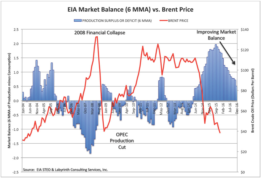
Oil enables constant world per capita productivity growth. As such, its real yield does not increase at the rate of productivity growth, but rather remains constant. The implication is that the supply and consumption of oil per capita has been constant.

Chart 14 indicates that this has held true at the World level for 45 years.

The expected real price of oil should remain constant over time: in fact, it does adjust for the CPI.

Chart 14: (author) Real USD$ price of oil

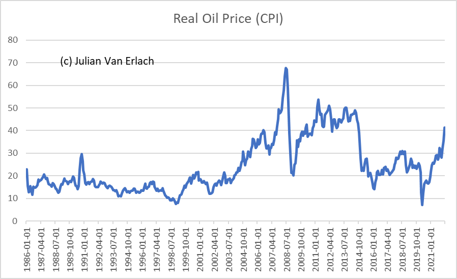
The USD$ index as measured by the DXY has also on average remained constant over this time; demonstrating that the above effect is not due to a rising US exchange rate pushing oil prices down.

Chart 15: (MacroTrends.com) DXY USD$ Exchange Rate

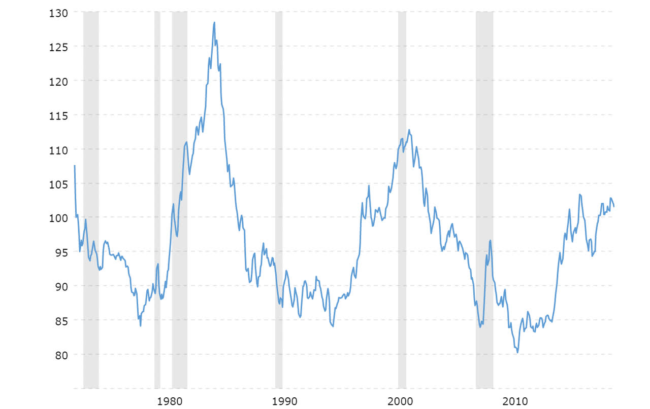
Investment Implications

Real Yield: if the Fed follows through with balance sheet reduction, the real yield will rise, putting downward pressure on gold, Bitcoin, and oil.

Inflation: baring policy change affecting the money supply, expected inflation will continue to decline which will drive the P/E up and put pressure on both gold and Bitcoin.

Earnings: recession and a fall in earnings is the wild card. If the scope of any expected earnings decline exceeds the P/E (valuation) favorability of falling inflation expectations, the stock market may fall further. An expected earnings decline would have to be well in excess of 14% to have a material impact on the market given the degree of apparent undervaluation of the current P/E vs. what the P/E should be at the current level of expected inflation.

Bond Yield: if the Fed continues reducing its balance sheet, in the context of NO recession, the rise in the real yield to a normal range of near 2% will offset falling expected inflation to drive nominal yields higher. A recession will delay this and would push real yields lower.

Intellectual Property Notice

Computer applications of the formulas described herein are subject to Patents protection: 8095444 and 7725374. Author may be contacted via LinkedIn.